In this passage, I will introduce a little more about the ‘prominence formation’ project.
-
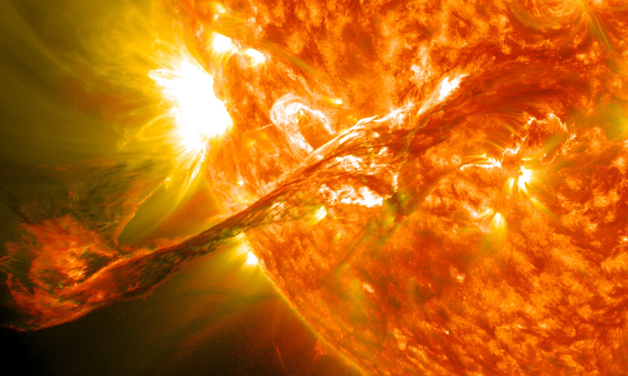
Solar Prominence
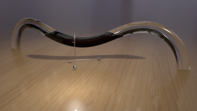
Solar prominences are cool and dense plasma suspending in the solar corona. Like the picture here.
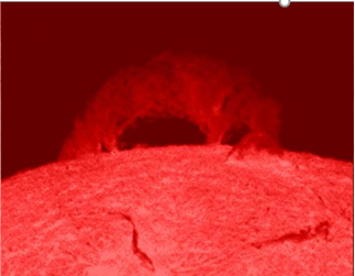
They are usually 100 times cooler and 100 times denser than the surronding environment.
Then, a straightforward question is, why such a heavy blob of plasma could float in the corona?
You might say that, well, it is similar with clouds floating in the air.
But actually it is different.
Although clouds are composed of water, their density are typically lower than the surronding atmosphere.
However, for solar pormineces, they are really heavy, 100 times denser. Why they can still float in the corona?
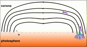
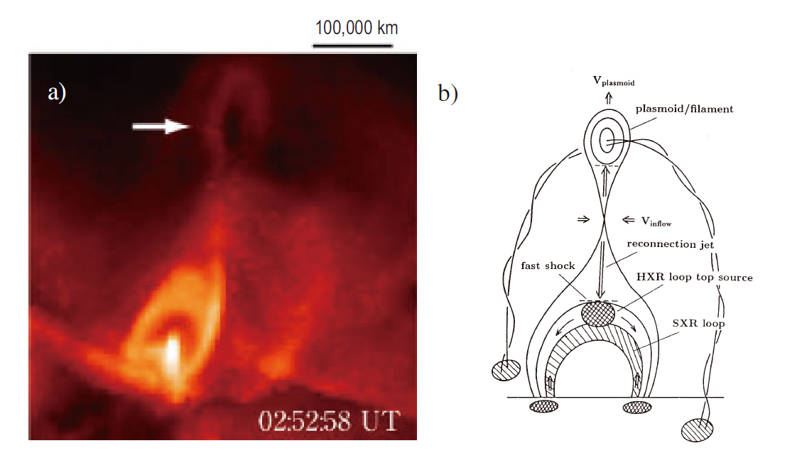
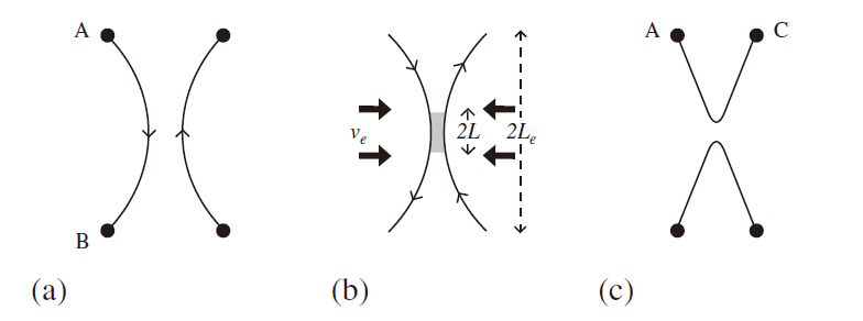
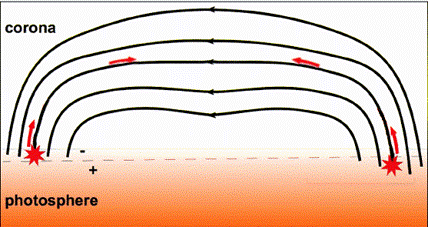
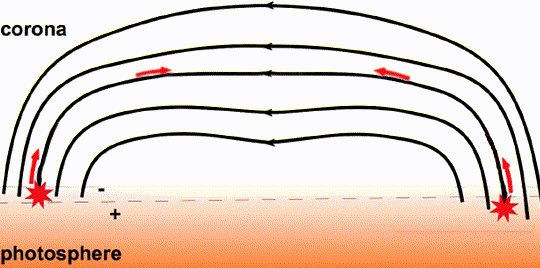
Nowadays, it is believed that, solar prominence are supported by the Lorentz force. On the earth, the magnetic field is weak. We cannot feel the effect of Lorentz forece in most situations. But on the sun, magnetic field is so stronge that the plasma could be supported by the Lorentz force. Especially in the solar corona, everything is dominated by the magnetic field, and the plasma is trapped inside the magnetic field. Suppose I have a magnetic line, like shown in the figure below. Then, plasma can only move along such a magnetic line, or we can call it a magnetic flux tube.

Then, it is easy to image that, if the magnetic field line has a upward dip, it is possible to support the heavy plasma, e.g., solar prominence.
However, here comes another question. Where does the (plasma forming the) prominence come from? How is these heavy plasma transported into the tenuous corona?
-
Evaporation–condensation model
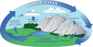
Well, you must know that the cloud on the earth is formed by evaporation and condensation. While for the prominence, though we have many mechanisms to explain that, one of the most popular mechanism is call evaporation and condensation model.
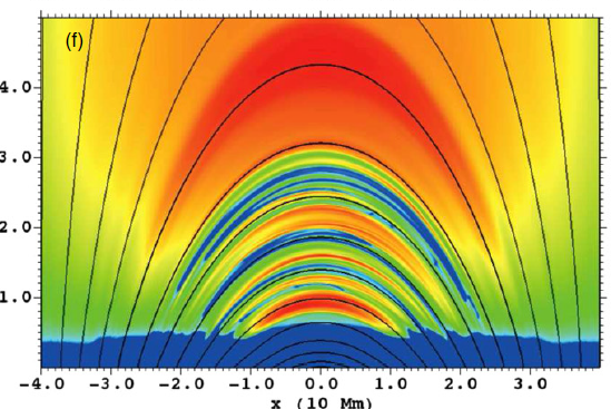
As shown in the GIF below. If I have a strong heating (caused by some activities in the lower atmosphere usually in the photosphere or chromosphere), at the footpoints of the magnetic field lines, plasma will be evaporated and then accumulated at the top of the magnetic field line. Here, condensation might happen because of a physical process called thermal instabiliy. So that we can see the formation of a cool and dense solar prominence.

So, what is thermal instabiliy?
Briefly, plasma will loose their energy, always everywhere. But note that we have a global heating in the corona (so that corona is always hotter than chromosphere, but the phycial essence of this global heating is still under debate), they can usually make a balance between the loss and the gain of the energy.
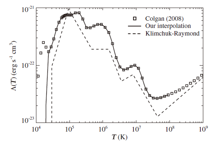
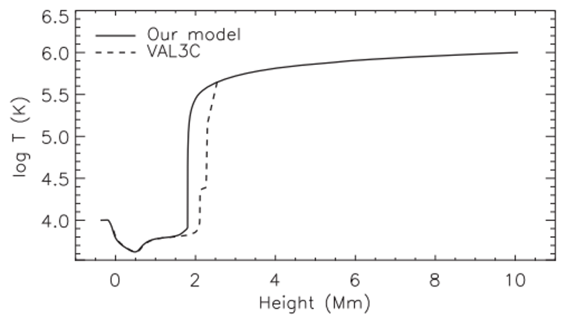
However, plasma at different temperature will lose their enery with different speeds. See the figure below. The dashed (or solid) curve, called cooling curve, describes how much energy plasma at a certain temperature will lose per second.
 Solar corona is usually at a temperature of 1 MK, e.g., 106 K. Then, suppose that plasma at 1 MK is suffered from some perturbation, and its temperature dropps to 0.99 MK. From the curve, you can see that it will lose more energy, while at the same time, the energy it gains from the global heating is (almost) not changed. So the balance is broken. It will lose more and more energy and become cooler and cooler. Such a catastrophic process is call thermal instabiliy.
-
Injection model
Another model, the injection model, is more straightforward. In this model, we also have an energetic event happens at the footpoint. But this time, the energetic event provides the plasma more momentum instead of thermal energy. Then, the cool plasma in the lower atmosphere is pushed up into the corona instead of being evaporated, as shown in the GIF below.
-
Unified model
From the previous description, we can find that, these two models are pretty similar. They both first have a heating/energetic event at the footpoint. And then, the plasma located in the chromosphere moves upward into the corona. The difference only existes in how much the energy is converted into kinetic energy or thermal energy.
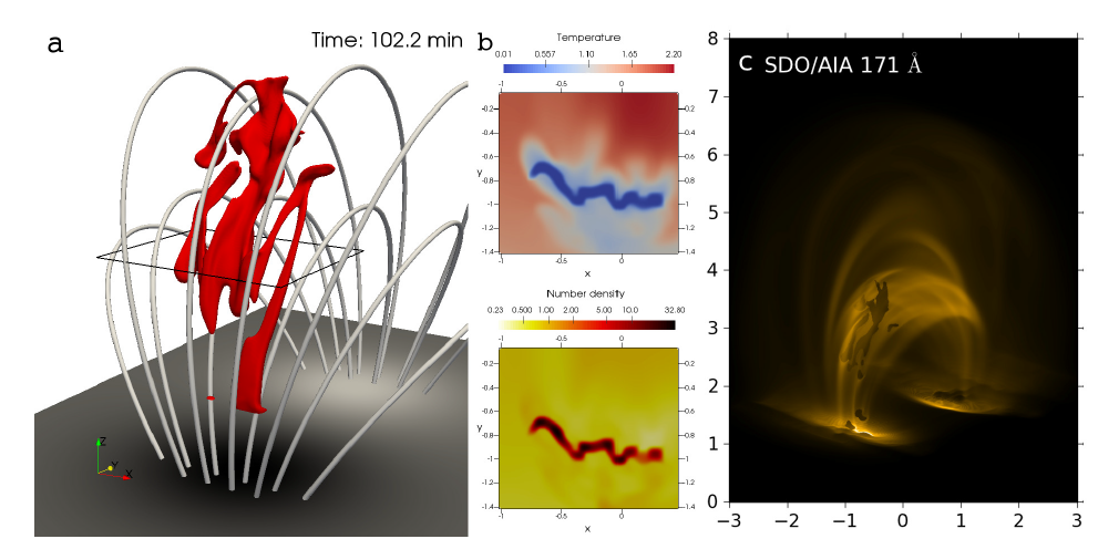
In recent work, a unified model is proposed. It points out that, these two models should be the same while the difference is that, in the evaportation–condensation model, the heating source is a little bit higher than in the injection model. That means, if the small energetic event happens in the lower corona or the higher chromosphere, it would more likely to be an evaportation–condensation prominence while an injection prominence would more prefer to a lower chromosphere energy source.
However, in their paper, the authors only provide two successful case with two paticular sets of parameters to demostrate their idea. We still want to check the model in a more detailed parameter space. For example, when keeping other paramters fixed, (the location of the energy source) from which height to which height, it would be an injection model, while from which height to which height, it would be an evaportation–condensation model; Or for a fixed height of energy source, whether the scale or duration of this will change the physical scenario. This is the idea of this project.
-
Run the test simulation in AMRVAC
In AMRVAC, we have a test code for the formation of solar prominece, based on the evaporation–condensation model.
Note that, again, everything happens in a 1D rigid tube, and plasma now could be understand as normal hydrodynaic fluid instead of MHD, a 1D hydrodynamic simulation is enough to simulate such a physcial process.
This code works in two stages.
First step, the code start from an hydrostatic equilibrium initial state, we only have a background global heating. We relax it to a thermal dynamic equilibrium state. This stage is from t=0 to t=200.
Second step, after we get an equilibrium tube, we start to add the strong heating at footpoint so that evaporation could happen. This stage is from t=200 to `time_max’ you input to the code (see below).
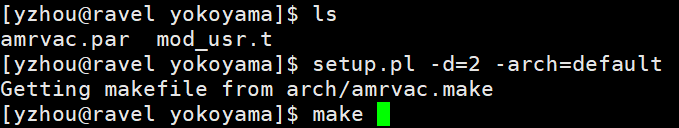
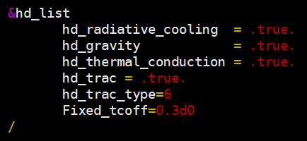
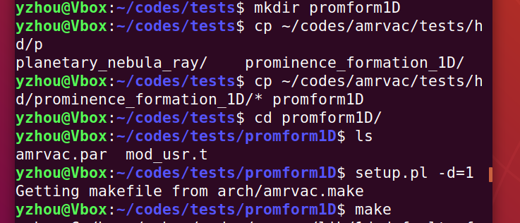
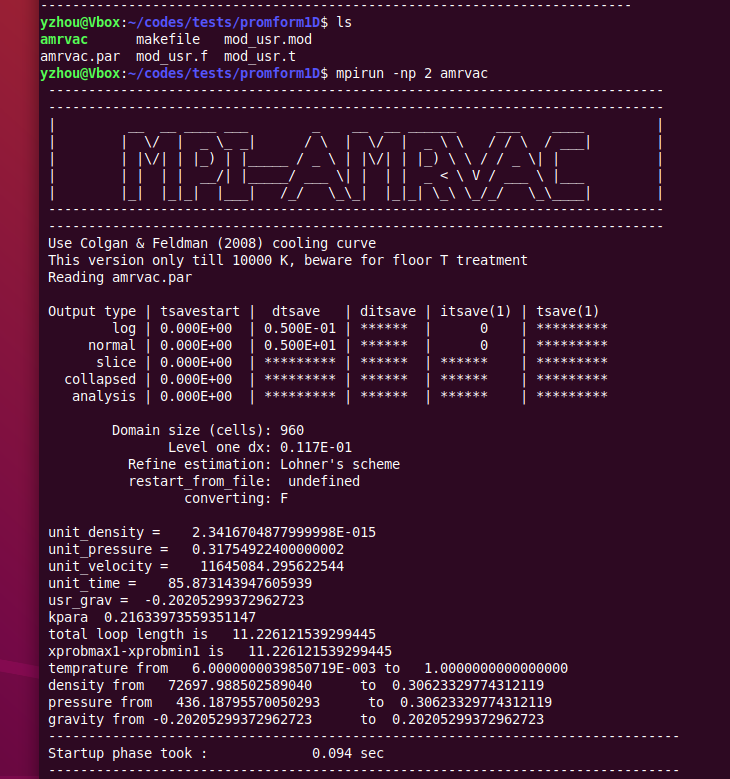
In the folder amrvac/tests/hd/prominence_formation_1D, you can find the mod_usr.t file and amrvac.par.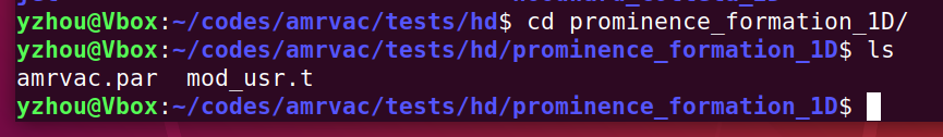
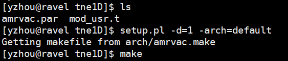
Copy them to your own folder, and use setup.pl to get the makefile and use make to complie it.
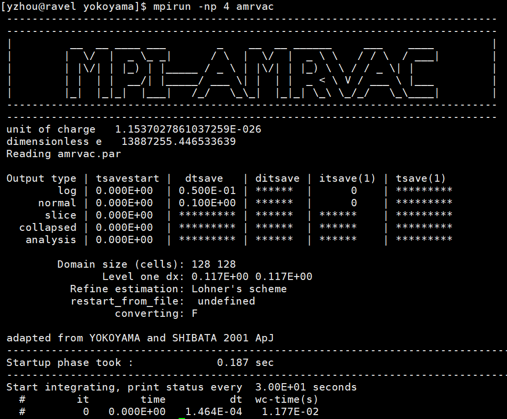
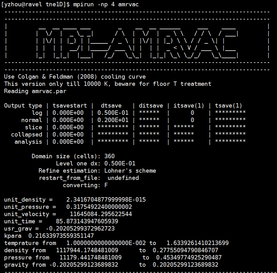
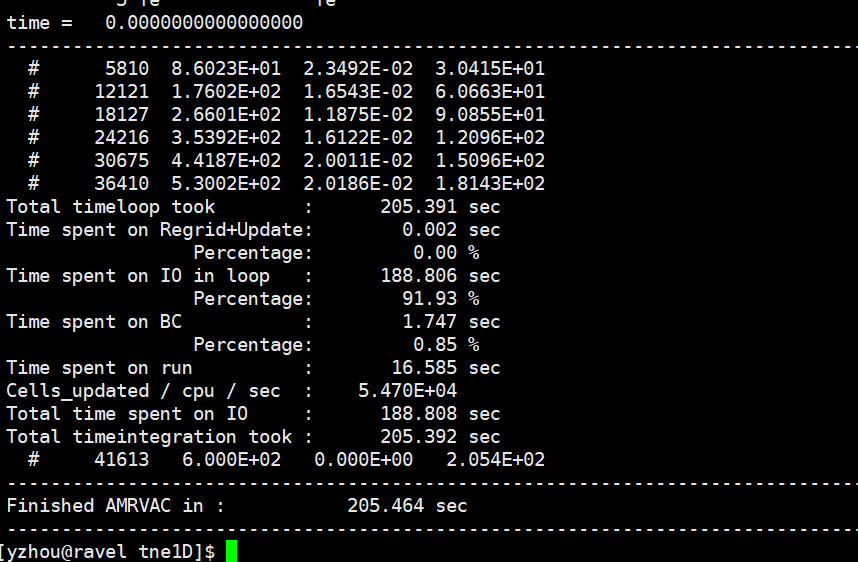
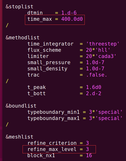
You can now run the code directly with the command mpirun -np 2 amrvac (here -np 2 means using 2 cores, you can use other numbers depending on your laptop). But before that, we have to change two lines in the amrvac.par file: time_max and refine_max_level. time_max = 400 is enough for this default setting. refine_max_level = 3 is already good enough, setting it to 4~6 would have a better result but will spend much more time.
Save the amrvac.par file and run the code.
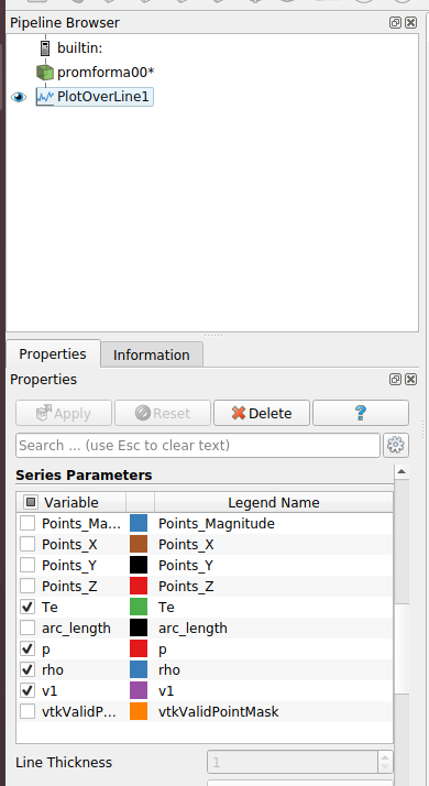
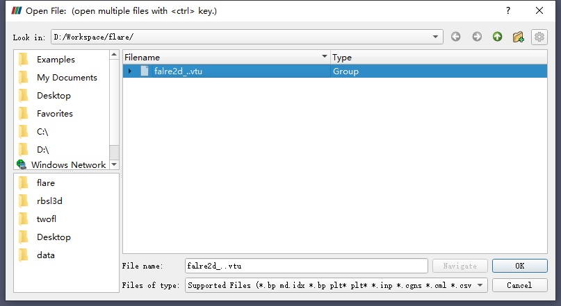
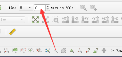
Now you can check the result with ParaView, OK and Apply (botton on the left side).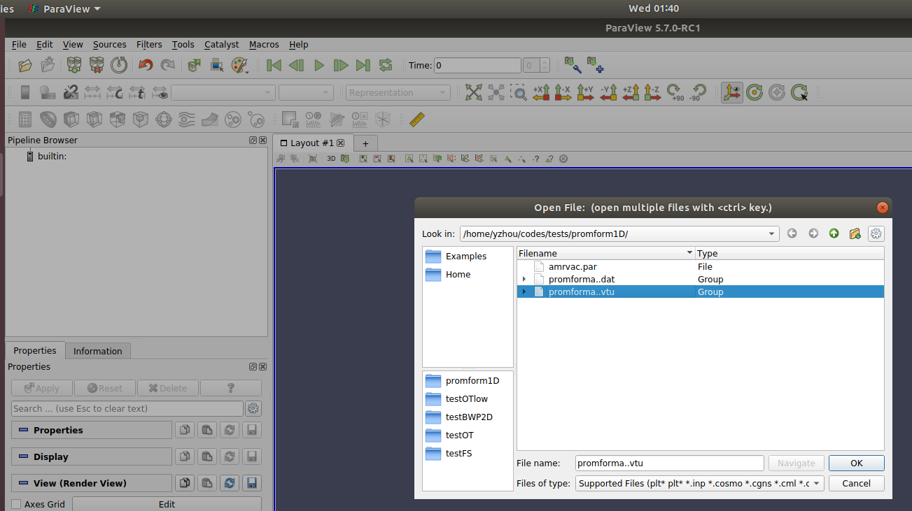
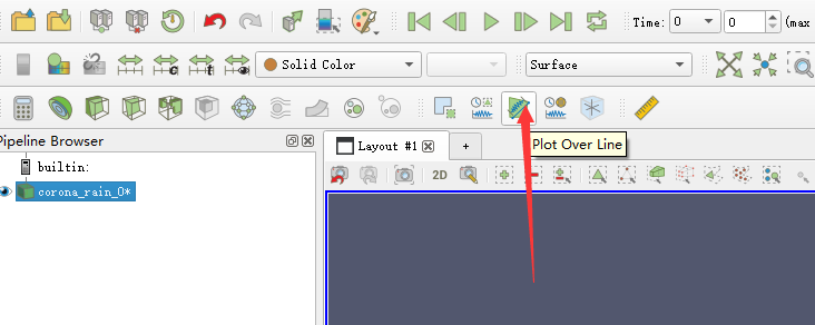
Use the plot over line tool, Apply.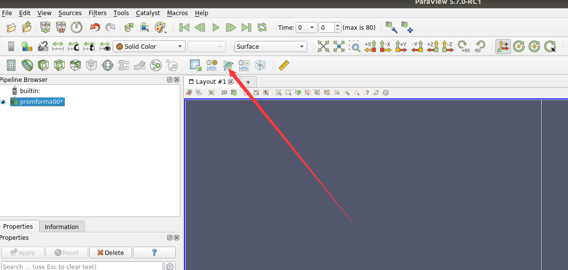
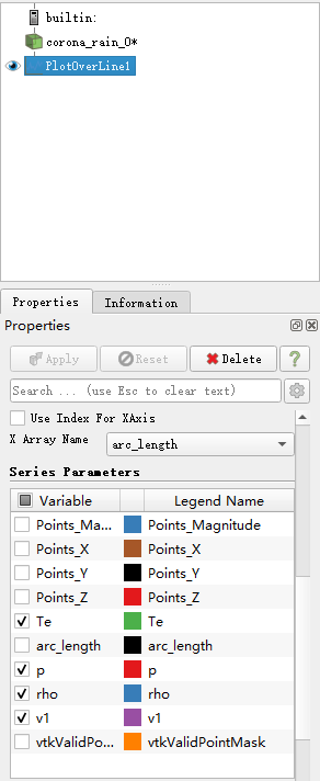
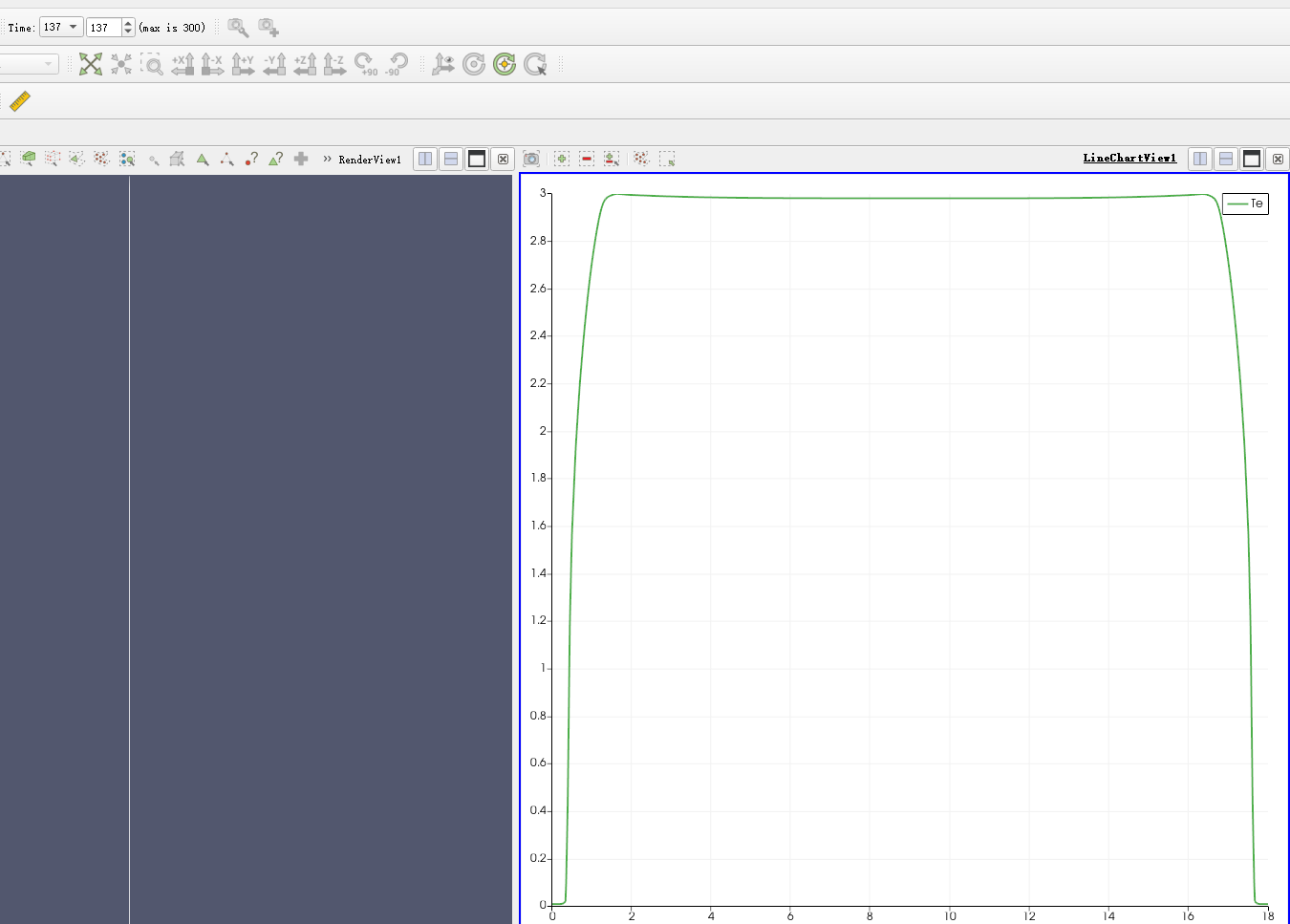
And then, on your left side, you can see all the avaliable variables. Here we choose Te, means temperature in the unit of 1 MK. (rho is number density in the unit of 10^9 / cm^3, p is pressure with the unit of 0.317 erg / cm^3, and v1 is velocity with the unit of 116.45 km/s.). Untick other variables.
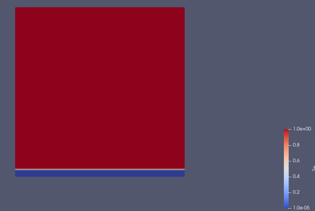
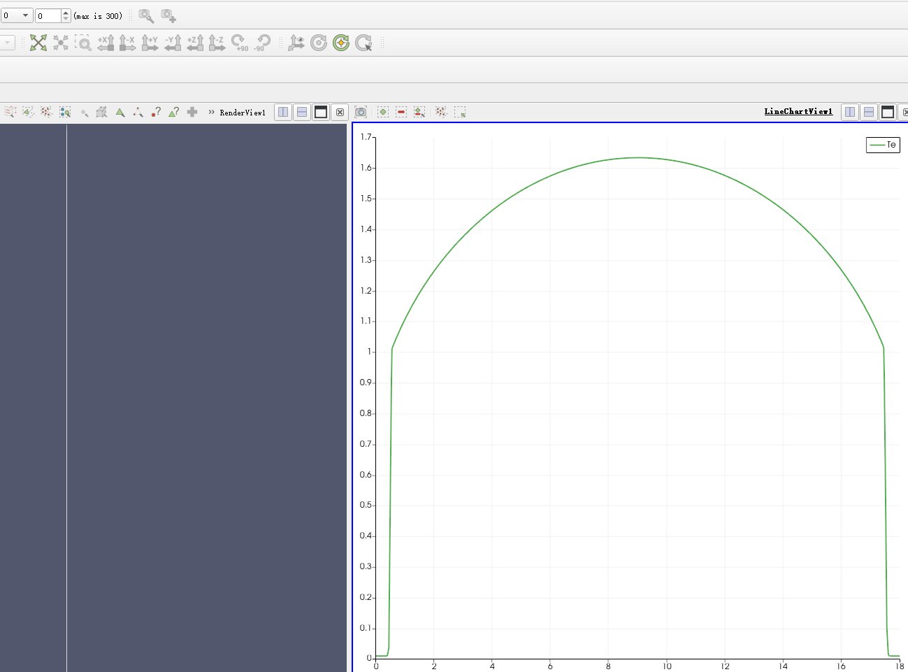
Then, on the right side, you can see the initial temperature distribution (along this 1D simulation domain, or this 1D rigid tube).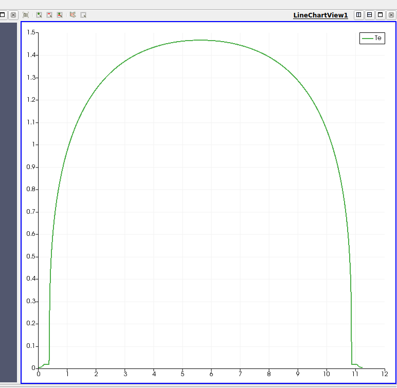
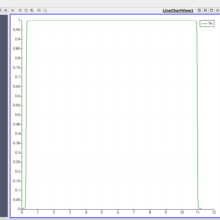
Find the time box on the top of the tool. Change it to 40. Since in the code, we save our snapshots every 5 time unit (controlled by the parameter dtsave_dat = 5.d0), the 40th snapshot should be t=40*5=200, e.g., the end of our first stage.
Here is the temperature profile at t=200, quite different with the initial one.
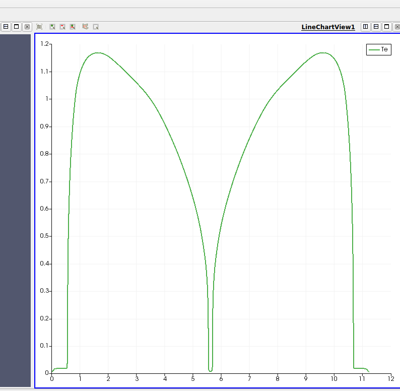
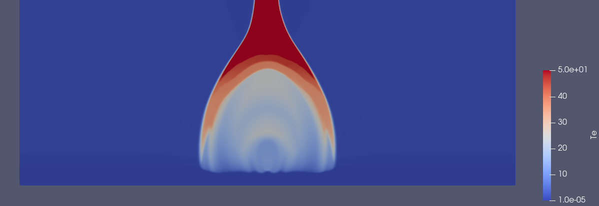
Then, in the second stage. With continous heating, you will find the temperature changes dramatically. And at the 52nd snapshot, you can already see that the temperature at the center drop down to 0.01, or 104 K. We have successfully got the prominence in the simulation.
-
Run the simulation of the injection model
As mentioned above, the test code is written for the evaporation–condensation model. If we want to simulate the injection model, we have to change the settings a little bit.
The most relavent part should be the subroutine getlQ (means get localized heating) in the mod_usr.t file.
You can read through this part and modify it according to the reference paper so that you can have a prominence formation using the injection model.
Remeber that, everytime you changed anything in mod_usr.t, you have to recompile the code (make again). While after changing amrvac.par, it is not necessary to do that.
-
Run the simulation of the injection mode
After reproduce what have already been done in the reference paper, we can move on to do a parameter survey, mainly on the height of the heating source (lH0), the duration of the heating source, the size of the heating source (lambda), the strength of the heating source (lQ0), etc. To see how these parametes will influence the formation mechanism.
Write down your resuls in your final report.
P.S. You can set the parameter dtsave_dat smaller to have more output snapshots.
P.S.2 ParaView is convenient, but Python can do more things. If you are familiar with Python, you can check the following links to see the Python tools in AMRVAC.
http://amrvac.org/md_doc_python_datfiles.html
http://amrvac.org/md_doc_python_vtkfiles.html
Good luck ~
 base_filename
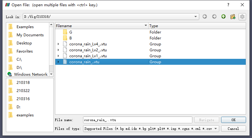


 Now you can check the result with ParaView, OK and Apply (on the left side).