Coronal Rain: 1D hydrodynamic simulation

In this passage, I will introduce a little bit more about the ‘1D corona rain’ project.

• Background

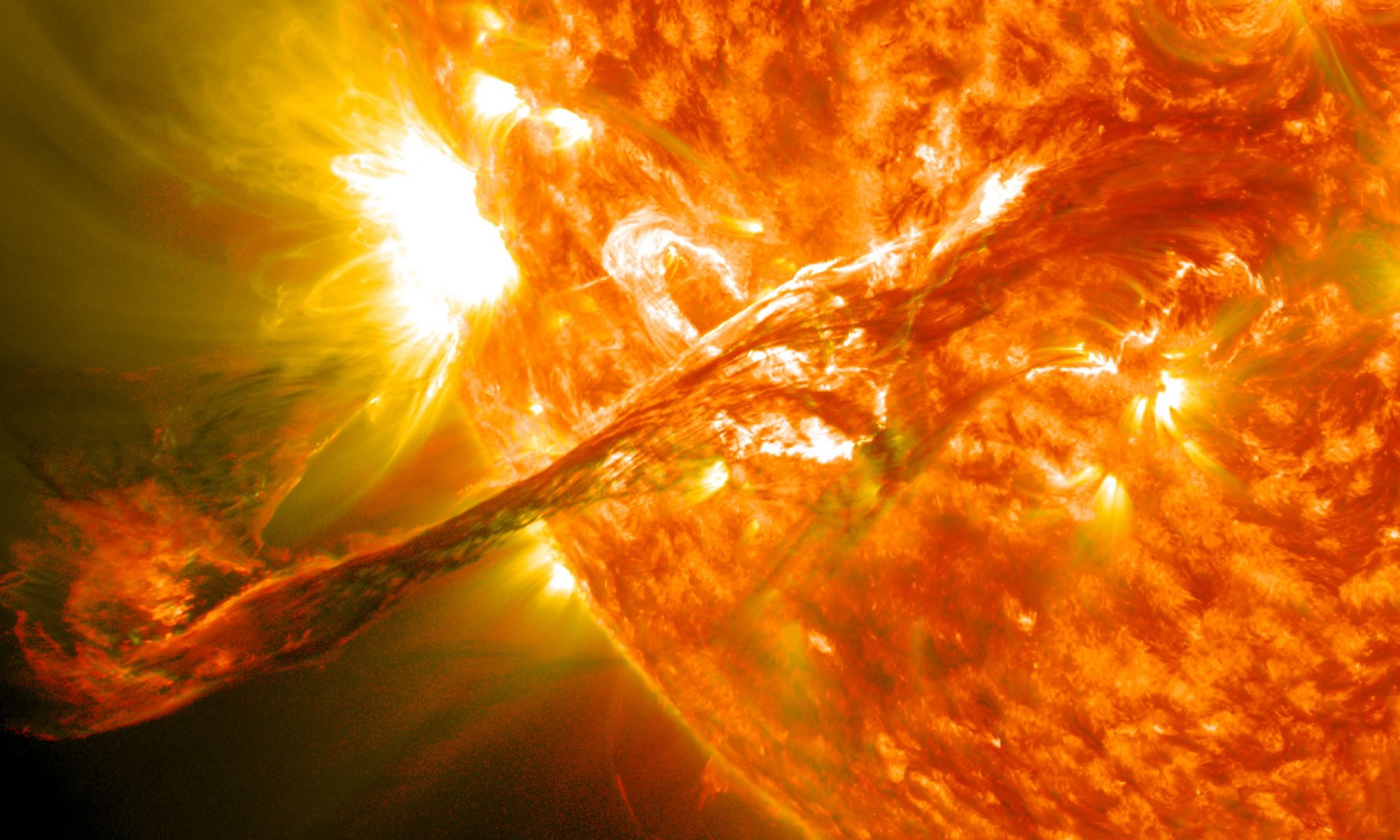
First, some physical background about coronal rain.

You can see some videos to get some impression on it, like https://www.nasa.gov/mission_pages/sdo/news/coronal-rain.html. This might be the most famous video about coronal rain.

So, what is coronal rain ? How does it form ?

On our earth, rain is a very common phenomena. Liquid water is heated and evaporated into water vapor. Water vapor will then condenses to form clouds and precipitates back to earth in the form of rain and snow.

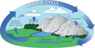
Coronal rain forms in a similar way. Plasma in the low atmosphere is cool and dense. It will be heated and evaporated up into the high corona. In the hot and tenuous corona, it will condense, becoming cool and dense again, and then fall back to the low atmosphere due to gravity.

The main difference between rain and coronal rain is the mechanism during the condensation. On the earth, water vapor condenses into clouds. That is simply because it is cooler in the high atmosphere than on the ground. But on the sun, the situation is different. The higher atmosphere, e.g., the solar corona, is much hotter than the low atmosphere, e.g., the chromosphere. The condensation is not directly due to the change of temperature.

Then, what is the mechanism for its condensation? That’s because of the radiation. Hot plasma will lose it energy due to radiation (usually noted as Λ(T), as function of temperature). In the equilibrium state, radiation is balanced by the continuous heating transferred from the low atmosphere. We call this heating background heating, which can help maintain the temperature of the solar corona. However, such an equilibrium is fragile. The following figure shows the radiation or the energy loss per unit volume, e.g., Lambda, as a function of temperature T. We can see that in the typical corona temperature (~1 MK), cooler plasma will lose more energy, which is different from our common sense.

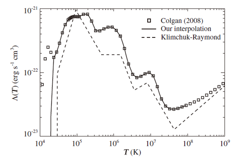
If we give the system a small perturbation, the temperature will drop a little bit. It becomes cooler. So it will lose more energy and becomes even cooler. Such a catastrophic process is the `thermal instability’. Thermal instability plays an important role in many phenomena in the solar corona, like coronal rain, solar prominences or some eruptive fall back blobs.

• Thermal Instability and Coronal Rain

We know that the sun has a much stronger magnetic field than the earth. In the solar corona, magnetic Lorentz force is much larger than some thermal forces like gas pressure. Consequently, MHD theory will tell us that motions in the solar corona is constrained or guided by the magnetic field line. Plasma can only move along the magnetic field lines, but cannot go cross. And its motions will have little influence to the magnetic field.

Given the above backgrounds, we can conclude the physical process into the following cartoon.

Here shows some magnetic field lines. We give some heating at the footpoints of the field lines. Plasma will then be evaporated into the high corona, cause a density perturbation in the corona. When the density is high enough or strictly the perturbation is high enough, thermal instability so that condensation will happen. The cool and dense plasma blob will form and then fall back to one of the footpoints of the field lines.

• Previous simulations

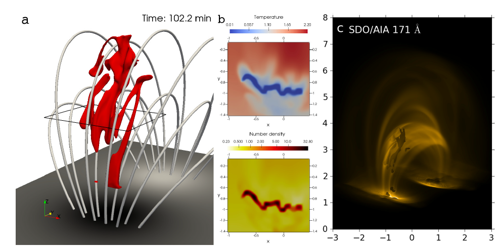
Such a mechanism has been demostrated by some recent 2D or 3D simulations. The following figures are from 2D and 3D simulations, respectively.

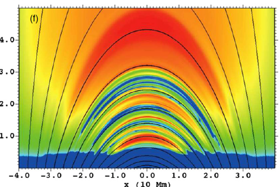
Remeber that plasma will always move along the magnetic field lines while their affect to the magnetic field lines is minor. Motions in different field lines are independent. Especially in the 2D case, you can see this very clearly. Thus, to explain such a physical process, we only need to pick out a single magnetic field line (which is called a magnetic flux tube) and simulate the motions inside the one-dimensional (1D) flux tube, like the cartoon here.

Actully, this kind of 1D simulation has been used for more than 20 years. Although nowadays, 2D or even 3D simulations of coronal rain are available. 1D simulations are still useful because in 1D simulations the resolution could be very high. We can look into some details.

• Problems and solutions

In 2D or 3D simulations, we often find that even after we add the heating for a long time, the condensation does not seem to happen. While for 1D simulation, the condensation can easily happen in most cases. Why?

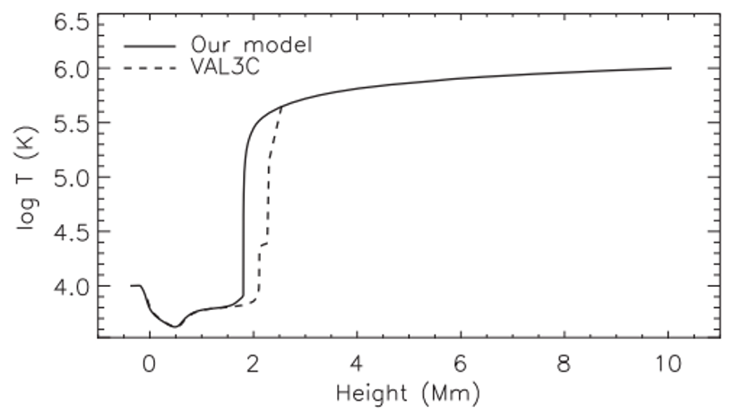
Previous works found that it should be related to the resolution. The following figure show how temperature evolves with height, starting from photosphere. Between the chromosphere and the corona, there is a thin layer called transition region (TR). In the TR, temperature increase quickly, which means the temperature gradient is large. And this region is crucial for the evaporation process. If the resolution is not enough, temperature gradient cannot be calculated correctly, the energy (strictly, enthalpy) conducted by thermal conduction will be wasted in the even lower chromosphere. And the final consequence is the evaporation will be underestimated, or in other words, the perturbation in the solar corona cannot be strong enough. As a result, thermal instability will fail to happen in some simulations.

But in 2D or 3D simulations, such a high resolution as 1D is currently not affordable. So can we still have a physically `correct’ result using a low resolution setting? Recent research made it possible. We can artificially broaden the TR by setting a global cutoff temperature T_c (typically ~250, 000 K). For the region where is cooler than T_c, thermal conduction and radiative cooling will be modified artificially. The result of such a modification will broaden the TR without significantly changing the coronal properties. And by such a broadening, even with a low resolution (that is available by current 2D or 3D simulations), the evaporation could be calculated correctly. We will call it TFix method hereafter.

But there is a small drawback for the TFix method, as pointed out by some recent works. In some cases, the characteristic temperature of the TR can change dramatically during the simulation, making it unclear how suitable a fixed value of T_c is for capturing the dynamic evolution of the system that are impulsively heated. That is why they proposed another method, called the TRAC (transition region adaptive conduction) method.

In the TRAC method, cutoff temperature T_c is determined dynamically with the evolution of the system, making the result more reliable. However, it also suffers from a problem that the TRAC method is originally designed for 1D simulation only. If we apply it in 2D or 3D simulations, we have to calculated different T_cs for different field lines, which needs plenty of computation and will slow down the simulation.

To conclude, the TFix method can handle some problems, and has the advantage of simple and quick. While the TRAC method is more precise in the cost of more time (in multi-dimensional simulations).

• Aim of the project

So, here is our question and the aim of the project. We want to know, in what kind of heating events, the TFix method can give reliable / acceptable results? While in what kind of heating events, the results given by the TFix method will deviate obviously from the result given by the TRAC method?

I will give you tens of different heating cases, corresponds to different types of heating, like steady heating, impulsive heating or even explosive heating. You should run each case by the TFix method and the TRAC method, respectively. And compare their results to see in which cases, two methods show similar results while in which cases, two methods show significately different results. For example, you can organize the results in a table:

No correction	TRAC	TFix (T_c=200,000 K)	TFix (T_c=300,000 K)	TFix (T_c=500,000 K)
case 1
case 2
case 3
case 4
case …

• Run the simulation

After you have correctly installed AMRVAC (for the installation of AMRVAC, you can check http://amrvac.org/ or the link mentioned in the first email), you can run some 1D tests in the tests folder.

Then you can start the simulation.

I will give you several files.

You need to

Move setdt.t and mod_global_parameters.t into amrvac/src/

Move mod_trac.t into amrvac/src/mhd/

Move mod_hd_phys.t into amrvac/src/hd/

To replace the files there.

Then, there are still 2 files, mod_usr.t and amrvac.par.

Create a new folder anywhere. And move these 2 files in this new folder. It would be your working directory.

mod_usr.t contains some subroutines for this project. In principle, it is not necessary to change anything in this file. But remember that once you have changed anything in this file, you use use the make command before you run a new simulation.

amrvac.par file contains some parameters used in the simulation. I will introduce a little bit more about the parameters here.

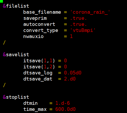base_filename is the output directory and name of the output .dat files. By default, the output files would be in the current directory. Rename it for different cases. If you want to output the files somewhere else, like ‘/volume/mysimulation/coronalran/case1_’, do remember that this directory should exist before you run the simulation.

time_max = 600.d0 means the simulation will run from t= 0 to t=600 unit_time. By default, 1 unit_time in the code corresponds to 85.875s, so 600 unit_time is 14.3 hrs. I think it should be suitable for most of the cases. You can change it if necessary.

autoconvert=.true. means AMRVAC will also output a .vtu file besides .dat files. .vtu fies could be visualized easily with Paraview (or other tools).

dtsave_dat = 2.d0 means AMRVAC will save the output files every 2.0 unit_time. If time_max=600, you will get 301 output .dat files.

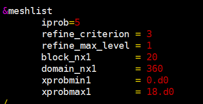
Here, iprob corresponds to different cases. iprob=1 corresponds to case 1, iprob=2 corresponds to case 2, etc. As mentioned in the previous email, cases are select from Table 1 in Johnston et al. 2019, A&A 625, A149. Do read the paper before you run the simulation.

xprobmin1=0 and xprobmax1=18 give the computational domain, e.g., x ranges from 0 to 18 unit_length. By default, unit_length is 10 Mm. That means x is from 0 to 180 Mm.

domain_nx1=360 means you have 360 level 1 grid cells in the simulation. That means your base resolution would be 180 Mm/360=500 km. Note that here we say level 1 grid. AMRVAC can adaptively refine the grids, the maximum refine level is set by refine_max_level. If refine_max_level=2, your effective resolution would be 500km/2=250 km, and if refine_max_level=3, it would be 250 km/2=125 km, etc. In this project, I think refine_max_level=1 or 2 should make the resultco resolution used in 3D simulation. Level 3 is not necessray.

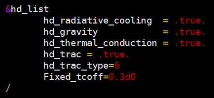
If hd_trac is false, the simulation will not use any correction.

If it is true, you have to set hd_trac_type. In this project, you have two choices, hd_trac_type=1 means using the TRAC method; hd_trac_type=6 means using the TFix method. And when using TFix method, you have to tell the code the fixed cutoff temperature T_c by setting Fixed_tcoff. By default, unit_temperature=1 MK. That means if you want to sett T_c=250,000 K, you have to set Fixed_tcoff=0.25.

OK, I think that’s all necessary information for this project.

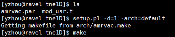
Then, you can compile the these two files as you did with the tests, using the following commands:

setup.pl -d=1 -arch=default

make

After successfully compling the code, you can run it by

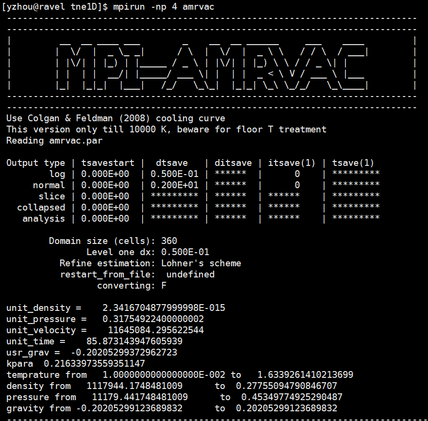
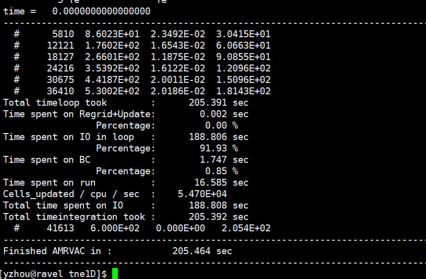
mpirun -np 4 amrvac

The parameter 4 after -np means using 4 cores. You can change it according to you machine.

• Analyze the results

You can have a quick look on the result by using Paraview (or other tools like Visit).

Load the vtu files and Apply (on the left side).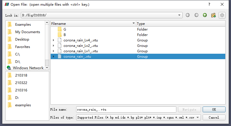

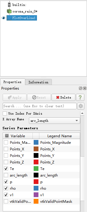
Using the tool “Plot Over Line”, and Apply.

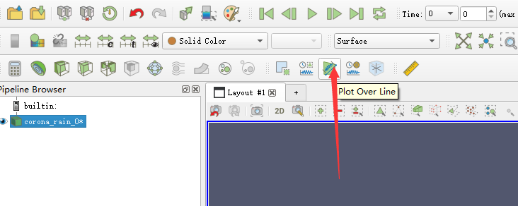
This tool will plot the distribution of some physcial quantities along the 1D coordinate. You can choose between Te (temperature), p (gas pressure), rho (density) and v1 (velocity). They are all shown as dimensionless quantities.

By default,

Te is in unit_temperature = 1 MK

p is in unit_pressure = 0.317538 dyn / cm**3

rho is in unit_density = 2.341668e-15 g / cm**3

v1 is in unit_velocity = 116.45 km/s

Take temperature for example, you can see the initial distribution of temperature.

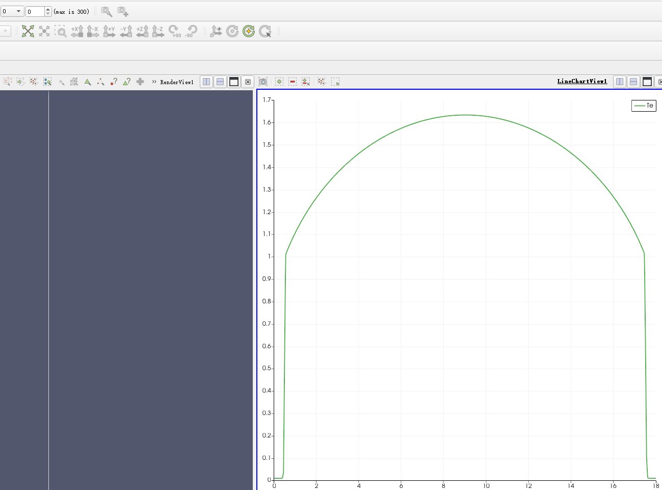
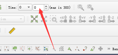
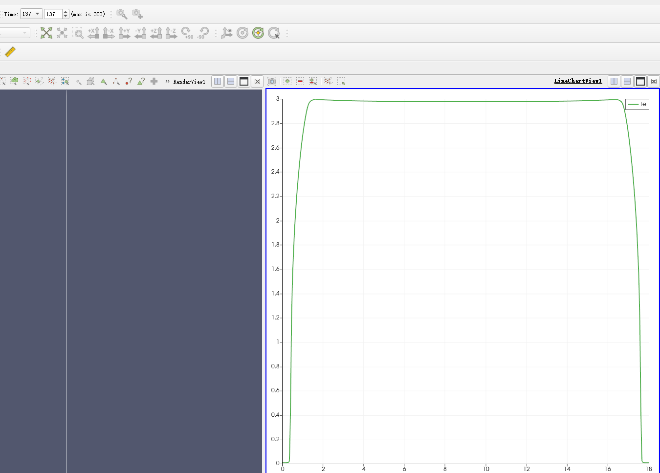
Note that you can change between different snapshots by change the “Time” on top of the menu bar.

So, here is temperature distribution at another time.

ParaView is convenient, but Python can do more things. If you are familiar with Python, you can check the following links to see the Python tools in AMRVAC.

http://amrvac.org/md_doc_python_datfiles.html

http://amrvac.org/md_doc_python_vtkfiles.html

Anyway, after you finish one case, you can change iprob, hd_trac and hd_trac_type. In this way, you can have results for diffrent cases. Compare the results and come to the conclusion.

Good Luck.