In this passage, I will introduce a little bit more about the ‘solar flare’ project.
-
Background
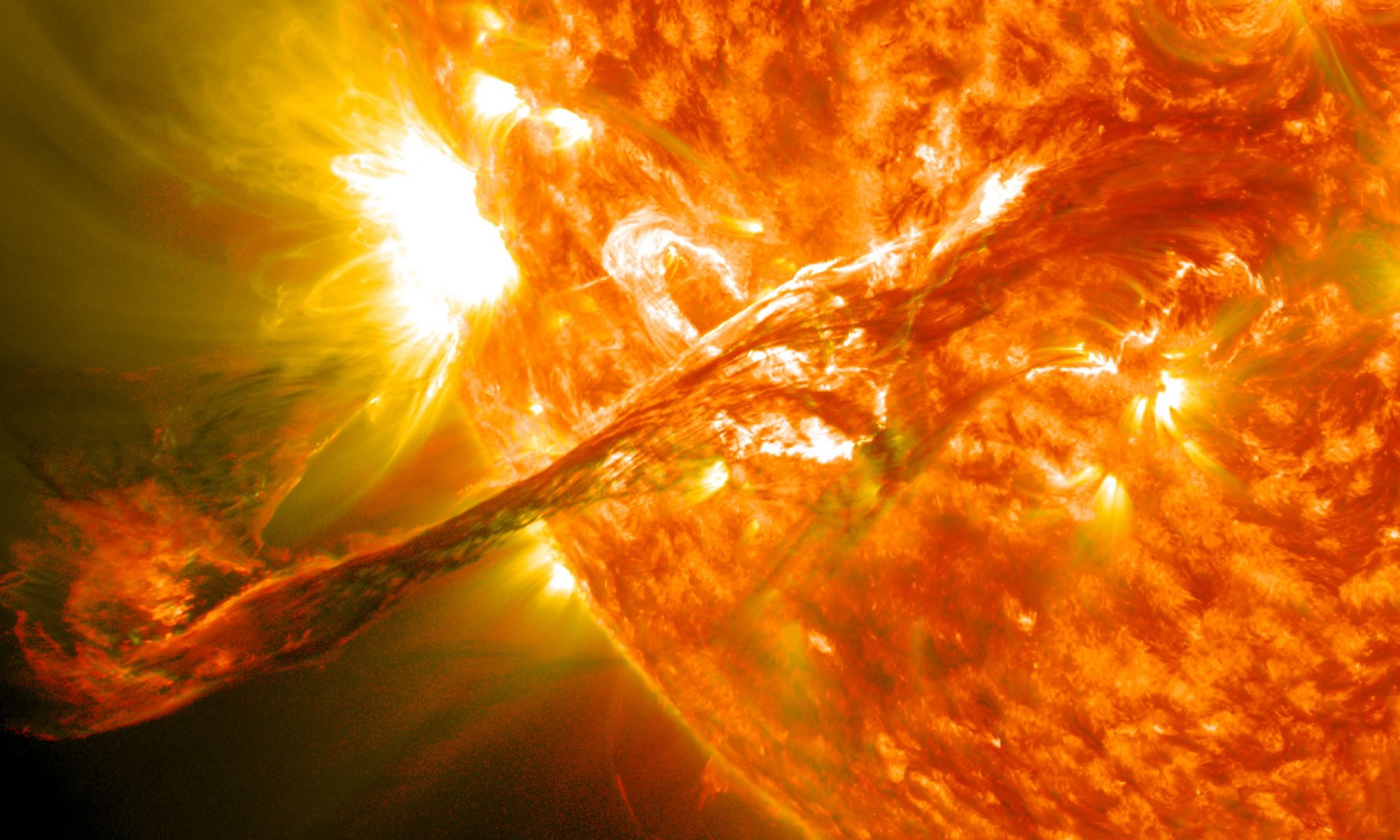
Solar flares are eruptive phenomena which often happen in the solar atmosphere, with up to 10^32 ergs of energy released within minutes. In a solar flare event, energy stored in coronal magnetic fields is directly or indirectly converted to thermal energy of plasma in the solar corona. Such a physical process is usually described by a standard flare model called CSHKP model (contributed by Carmichael, Sturrock, Hirayama, Kopp and Pneuman).
Horizontal convection beneath the photosphere will change the topology of coronal magnetic fields, e.g., the kinetic energy is turned into magnetic energy stored in the magnetic field. The energy could be release in many ways. One of these ways is magnetic reconnection.
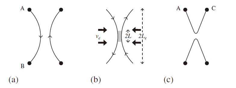
Sometimes, the magnetic field in the solar corona can form a structure named current sheet, a thin current-carrying layer across which the magnetic field changes either in direction or magnitude or both. The current sheet is not stable, as ohmic heating efficiently dissipates magnetic field inside it, the topology of magnetic field would be changed, as shown in the following cartoon. Such a physical process which breaks and reconnects of oppositely directed magnetic field lines in a plasma is called magnetic reconnection.
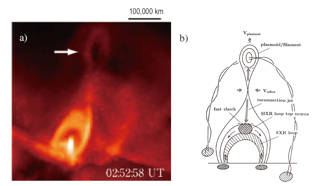
Magnetic reconnection is the crucial part of the CSHKP model. The released energy will generate a upflow and a downflow. The upflow is sometimes associated with an eruptive solar prominence/filament or CME. While the downflow jet will first hit the apex of the loop system beneath the current sheet, creating a bright hard X-ray source. And subsequently the downflow continuously goes down following the loop until down to the chromosphere, leading to a bright X-ray source at the footpoint. Such an energy flow will again cause evaporations in the chromosphere, which will heat the solar corona as well as the loop.
As many other physical processes happening on the Sun, magnetic reconnection could be described by both magnetohydrodynamic (MHD) models and kinetic models. Here, we will use only the MHD model for simplicity. In the MHD model, magnetic reconnection is mainly related to the induction equation, which could be derived from Faraday’s equation in combination with Ampere’s law and Ohm’s law, and you can see many other equivalent forms of this equation in literatures.
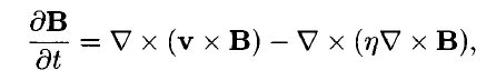
The ohmic heating is resulted from eta, the magnetic resistivity or magnetic resistivity, in right hand side of the equation. It is an interesting parameter. For a collisional plasma with strong magnetic field but a relatively weak electric field, the magnetic diffusivity is approximately given by Spitzer’s formula (see Spitzer 1962, Schmidt 1966).
However, measurements in laboratory experiments and computer simulations have shown that under certain conditions, the resistivity of a plasma tends to be much higher than the Spitzer resistivity. We call them anomalous resistivity. And from observations, we can neither know the detailed value of resistivity. So, in numerical simulation, we can only use values according to our experience.
In this project, we will run a typical numerical simulation on magnetic reconnection during solar flares, based on the work of Yokoyama & Shibata in 2001. And see what will happen with different resistivities. Usually, a lower resistivity will result in a slower reconnection, a low temperature of the reconnected loop, etc.
-
Run the simulation
After you have correctly installed AMRVAC (for the installation of AMRVAC, you can check http://amrvac.org/ or the passage The Installation of AMRVAC in this site), you can run some 1D tests in the tests folder.
Then you can start the simulation.
I will give you 2 files, mod_usr.t and amrvac.par.
Create a new folder anywhere. And move these 2 files in this new folder. It would be your working directory.
mod_usr.t contains some subroutines for this project. In principle, it is not necessary to change anything in this file. But remember that once you have changed anything in this file, you use use the make command before you run a new simulation.
amrvac.par file contains some parameters used in the simulation. I will introduce a little bit more about the parameters here.
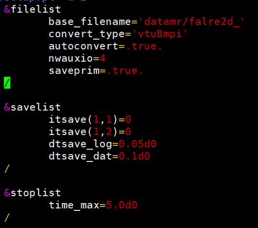
base_filename is the output directory and name of the output .dat files. By default, the output files would be in the current directory. Rename it for different cases. If you want to output the files somewhere else, like ‘/volume/mysimulation/flare/case1_’, do remember that this directory should exist before you run the simulation.
time_max = 5.d0 means the simulation will run from t= 0 to t=5 unit_time. By default, 1 unit_time in the code corresponds to 85.875s, so 5 unit_time is 429s. You can change it if necessary.
autoconvert=.true. means AMRVAC will also output a .vtu file besides .dat files. .vtu fies could be visualized easily with Paraview (or other tools).
dtsave_dat = 0.1d0 means AMRVAC will save the output files every 0.1 unit_time. If time_max=5.0, you will get 51 output .dat files.
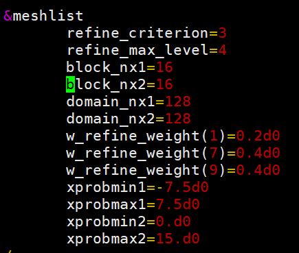
xprobmin1=-7.5 and xprobmax1=7.5 (and also xprobmin2/xprobmax2) give the computational domain, e.g., x ranges from -7.5 to 7.5 unit_length while y goes from 0 to 15.0. By default, unit_length is 10 Mm. That means the domain is 150 Mm x 150 Mm.
domain_nx1=128 means you have 128 level 1 grid cells in the x direction in the simulation. That means your base resolution in the x direction would be 150 Mm/128=1172 km. Note that here we say level 1 grid. AMRVAC can adaptively refine the grids, the maximum refine level is set by refine_max_level. If refine_max_level=2, your effective resolution would be 1172 km/2=586 km, and if refine_max_level=3, it would be 586 km/2=293 km, etc. In this project, I think refine_max_level=3 or 4 is OK.
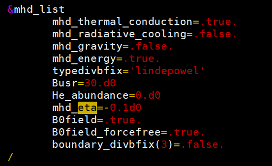
mhd_eta is the magnetic resistivity. You need to change this value and run different simulation. I recommend first trying these 5 values: 0.00002, 0.0002, 0.002, 0.02, 0.2.
Busr in this mhd_list controls the magnetic field strength. If necessary, you can also play with it.
OK, I think that’s all necessary information for this project.
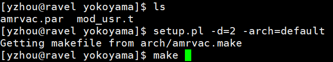
Then, you can compile the these two files as you did with the tests, using the following commands:
setup.pl -d=2 -arch=default
make
After successfully compiling the code, you can run it by
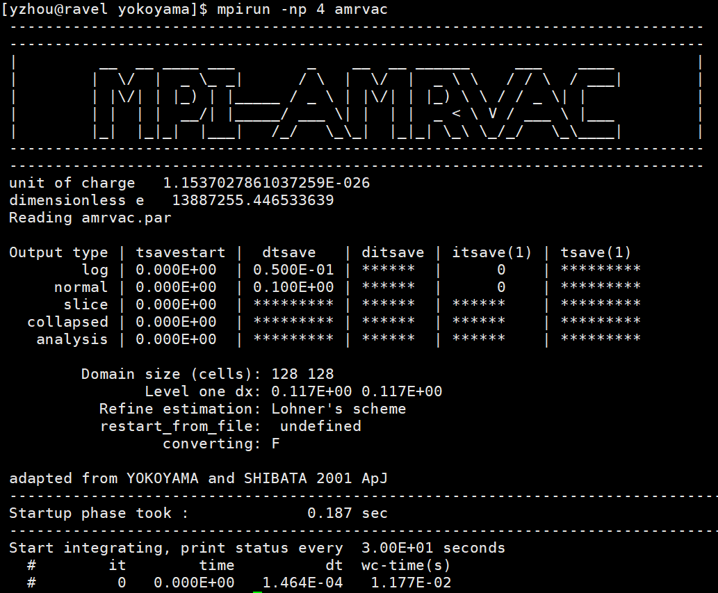
mpirun -np 4 amrvac
The parameter 4 after -np means using 4 cores. You can change it according to your machine.
-
Analyze the results
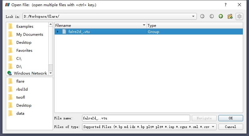
You can have a quick look on the result by using Paraview (or other tools like Visit if you are more familiar with them).
Load the .vtu files and Apply (on the left side).
You can then choose the physical parameter you want to check through the pull-down menu. Te is temperature, b1/b2/b3 are magnetic field bx/by/bz, j1/j2/j3 are corresponding current density, p is thermal pressure, rho is density and v1/v2/v3 are velocity vx/vy/vz.
By default,
Te is in unit_temperature = 1 MK
p is in unit_pressure = 0.317538 dyn / cm**3
rho is in unit_density = 2.341668e-15 g / cm**3
v1 is in unit_velocity = 116.45 km/s
b1 is in unit_magneticfield = 2 G
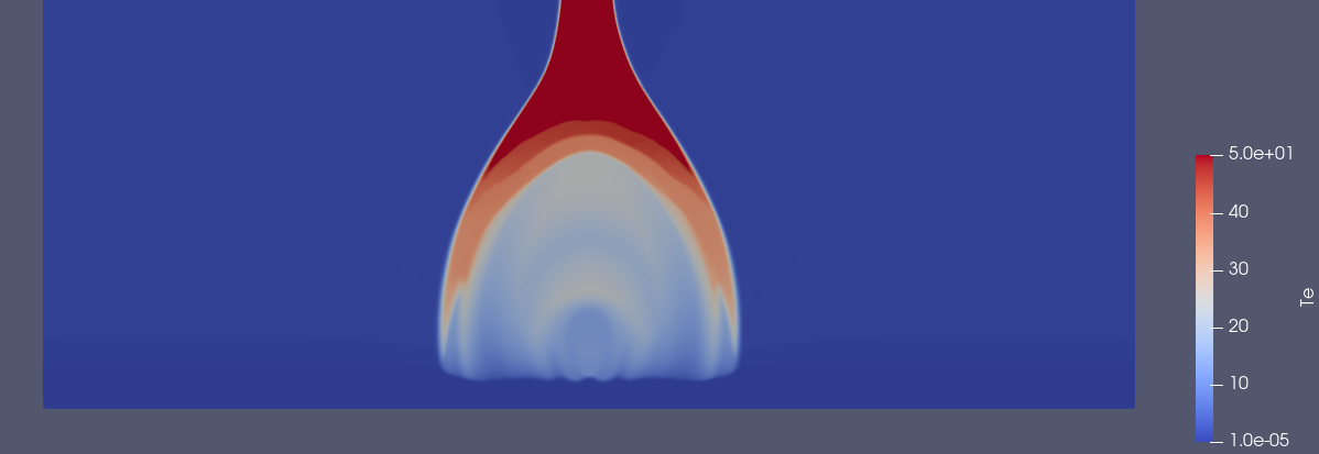
Usually, we will first pay attention to temperature in this case. So choose Te and you will see the distribution of temperature.

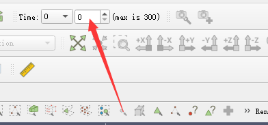
Note that you can change between different snapshots by change the “Time” on top of the menu bar.
So, here is temperature distribution at another time. We can see the formation of the reconnected hot loop.
After you finish one case, you can change mhd_eta and run another case. In this way, you can have results for different cases. Compare the results and come to the conclusion. For example, the time evolution of the temperature at the reconnetion region should be quite different for different mhd_eta. Anyway, with the results, there are many things worth analyzing further.
ParaView is convenient, but Python can do more things. If you are familiar with Python, you can check the following links to see the Python tools in AMRVAC.
http://amrvac.org/md_doc_python_datfiles.html
http://amrvac.org/md_doc_python_vtkfiles.html
Good Luck.